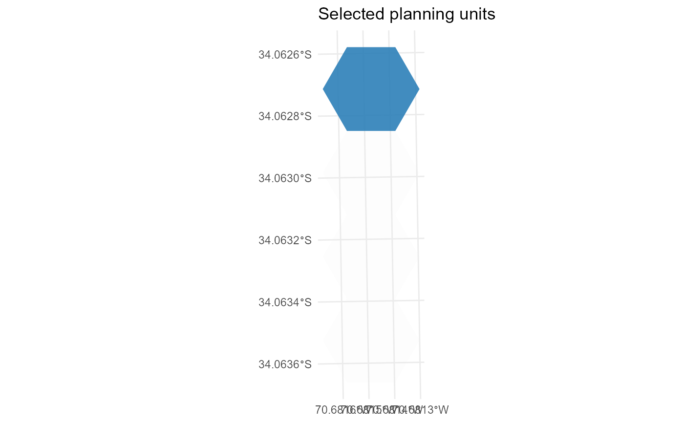
Plot the spatial distribution of selected planning units from a
solutionset-class object returned by solve.
This function maps the planning-unit selection summary returned by
get_planning_units onto the planning-unit geometry stored in
the associated Problem object.
Usage
plot_spatial_planning_units(
  x,
  solutions = NULL,
  ...,
  base_alpha = 0.1,
  selected_alpha = 0.9,
  base_fill = "grey92",
  base_color = NA,
  selected_color = NA,
  draw_borders = FALSE,
  show_base = TRUE
)
Arguments
- x
A
solutionset-classobject returned bysolve.- solutions
Optional integer vector of solution ids. If
NULL, the first available solution is plotted by default.- ...
Reserved for future extensions.
- base_alpha
Numeric value in \([0,1]\) giving the alpha of the base planning-unit layer.
- selected_alpha
Numeric value in \([0,1]\) giving the alpha of the selected planning-unit layer.
- base_fill
Fill colour for the base planning-unit layer.
- base_color
Border colour for the base planning-unit layer.
- selected_color
Border colour for selected planning units.
- draw_borders
Logical. If
FALSE, borders are not drawn.- show_base
Logical. If
TRUE, draw the base planning-unit layer underneath the selected units.
Details
Let \(w_i \in \{0,1\}\) denote the planning-unit selection variable for
planning unit \(i\). This function plots the user-facing
selected == 1 representation of \(w_i\).
If several runs are requested, the output is faceted by run_id.
Planning-unit geometry must be available in the associated problem object.
See also
get_planning_units,
plot_spatial_actions,
plot_spatial_features,
plot_spatial_planning_units
Examples
if (
  requireNamespace("sf", quietly = TRUE) &&
  requireNamespace("ggplot2", quietly = TRUE) &&
  requireNamespace("rcbc", quietly = TRUE)
) {
  # Load a complete simulated planning problem.
  example_data <- load_sim_multiaction()

  problem <- create_problem(
    pu = example_data$planning_units,
    features = example_data$features,
    dist_features = example_data$dist_features,
    cost = "cost"
  ) |>
    add_actions(
      example_data$actions,
      cost = example_data$action_costs
    ) |>
    add_effects(
      example_data$effect_assumptions
    ) |>
    add_constraint_targets_relative(0.05) |>
    add_objective_min_cost(alias = "cost", include_pu_cost = FALSE) |>
    add_objective_max_effect(alias = "benefit") |>
    set_method_weighted_sum(
      aliases = c("cost", "benefit"),
      runs = set_runs_grid(n = 3),
      normalize_weights = TRUE
    ) |>
    set_solver_cbc(verbose = FALSE)

  solutions <- solve(problem)

  plot_spatial_planning_units(solutions)
}