
Multi-objective forest restoration planning in a highly productive landscape
Source:vignettes/Integrated_planning.Rmd
Integrated_planning.RmdOverview
Restoration planning is especially difficult in highly productive landscapes. Most land is already committed to agriculture, forestry, or other economically valuable uses, so restoration cannot be treated as though it were being placed on vacant land. Every new restoration site competes with an existing use, requires public or private expenditure, and may alter areas that already provide important ecosystem services.
At the same time, ecosystem-service provision is often uneven across the landscape. Some locations already store substantial carbon, regulate water flows, retain sediment, or support biological control, whereas other locations provide comparatively little of these functions. In this example, the planning goal is therefore not to restore the sites with the highest current service values. Instead, it is to identify eligible sites with relatively low baseline levels of ecosystem services. These low-service locations are interpreted as areas of current ecological deficit where restoration may be most justified, while avoiding the displacement of functions that are already being supplied elsewhere.
This creates a genuine many-objective problem. A site with low carbon stock may still have high seasonal water yield, and a site with low sediment retention may be important for rodent and lagomorph control. Moreover, the least expensive sites are not necessarily those with the largest ecosystem-service deficits. Collapsing the four services into a single index would hide these conflicts and would require fixed exchange weights before decision makers have seen their consequences.
This vignette uses multiscape to extend an existing
conservation network with a fixed amount of forest restoration. Existing
conservation areas are treated as prior commitments and remain
unchanged. The optimizer decides where to add restoration within the
surrounding productive matrix while balancing five separate objectives:
implementation cost and the deficits to common service ceilings in the
selected restoration portfolio.
The example addresses the following planning question:
Which additional sites should be restored to complete the landscape commitment at low cost, while directing restoration towards locations with comparatively low current provision of multiple ecosystem services?
The analysis produces a set of alternative spatial plans rather than one predefined answer. These alternatives show how the restoration pattern changes when greater emphasis is placed on different ecosystem-service deficits.
Planning formulation
Let \(i \in \mathcal{I}_R\) index planning units that are eligible for forest restoration. The binary decision variable \(r_i\) equals one when unit \(i\) is selected for restoration and zero otherwise. The existing conservation network is fixed in every solution. It provides the spatial foundation of the plan, but the decisions compared in this vignette concern only the additional restoration units.
The total restoration cost is
\[ C(r)=\sum_{i \in \mathcal{I}_R}c_i^R r_i, \]
where \(c_i^R\) is the local cost of restoring unit \(i\).
For each ecosystem service \(f\), define a common ceiling \(M_f\) as the largest reference amount observed in the eligible restoration units. The effect assigned to restoration is the deficit to that ceiling:
\[ \Delta_{if}=M_f-q_{if},\qquad B_f(r)=\sum_{i\in\mathcal{I}_R}(M_f-q_{if})r_i. \]
Here \(q_{if}\) is the reference amount currently provided by unit \(i\). The four service objectives maximize \(B_f\), while implementation cost is minimized. A larger benefit means that restoration is allocated to a stronger current deficit relative to the common ceiling.
The complete objective vector is
\[ \left\{\min C(r),\ \max B_{\mathrm{control}}(r), \max B_{\mathrm{carbon}}(r),\ \max B_{\mathrm{water}}(r), \max B_{\mathrm{sediment}}(r)\right\}. \]
Every plan restores exactly \(K\) equal-area units. Consequently,
\[ B_f(r)=K M_f-\sum_i q_{if}r_i. \]
The first term is constant across plans. Maximizing this deficit therefore preserves the former criterion of minimizing current service provision in the restoration portfolio. This equivalence requires fixed effort, a common ceiling within each feature, and one restoration action per unit. It does not apply automatically to varying restoration effort or concurrent restoration actions.
The ceiling is an explicit accounting assumption for deficit-based
prioritization. It is not an estimated ecological response to
restoration. A low current value does not establish that a site can
reach the ceiling or will respond more strongly than another site.
Applications with estimated outcomes should supply those estimates to
add_effects() instead.
The four services remain separate objectives because their spatial patterns differ; no exchange weights between services are imposed in advance.
Landscape and ecosystem-service data
The example represents a highly productive landscape divided into 30,496 planning units. Within this matrix, only a subset of units is available for new forest restoration, while other units are already conserved or excluded from intervention.
Four normalized raster layers describe current ecosystem-service
provision: rodent and lagomorph control, carbon stock, seasonal water
yield, and sediment retention. Raster-cell values range from 0 to 1
within each layer. create_problem() sums these values
inside each planning unit, so the stored reference amounts can exceed 1.
Higher values indicate stronger current provision of the corresponding
service; lower values indicate areas where that service is comparatively
weak and where restoration may help address an existing ecological
deficit.
library(multiscape)
library(dplyr)
library(ggplot2)
library(terra)

service_data <- load_ecosystem_services()
planning_units <- service_data$planning_units
ecosystem_services <- service_data$feature_raster

service_labels <- c(
  L1_control_inv = "Rodent and lagomorph control",
  L1_stock_inv = "Carbon stock",
  L1_rend_inv = "Seasonal water yield",
  L1_reten_inv = "Sediment retention"
)

nrow(planning_units)
#> [1] 30496
names(ecosystem_services)
#> [1] "L1_control_inv" "L1_stock_inv"   "L1_rend_inv"    "L1_reten_inv"
The maps show that the four deficits do not occur in the same places. An area with low carbon stock may not have low water yield, and an area with weak sediment retention may still contribute substantially to biological control. This lack of spatial congruence is the central reason for retaining four separate objectives. A restoration plan that performs well for one service can still redirect intervention towards high-value areas for another.
names(ecosystem_services) <- unname(service_labels[names(ecosystem_services)])
terra::plot(ecosystem_services)
Define the restoration decision context
The planning-unit attributes divide the landscape into three
management roles. Units marked locked_in constitute the
existing conservation network and are included in every plan. Units that
are neither locked in nor locked out form the candidate pool for
additional forest restoration. Units marked locked_out are
unavailable because of land-use, institutional, or other planning
restrictions represented in the example.
The action table includes both conservation and restoration so that the final maps display the complete intervention system. However, only restoration is a variable decision. The conservation network is inherited from previous policy commitments and remains spatially fixed across all solutions.
planning_attributes <- planning_units |>
  sf::st_drop_geometry() |>
  select(id, cost, area, locked_in, locked_out)

actions <- data.frame(
  id = c("conservation", "restoration"),
  name = c("Conservation", "Restoration")
)

conservation_units <- planning_attributes |>
  filter(locked_in) |>
  transmute(pu = id, action = "conservation")

restoration_units <- planning_attributes |>
  filter(!locked_in, !locked_out) |>
  transmute(pu = id, action = "restoration")

feasible_actions <- bind_rows(
  conservation_units,
  restoration_units
)

action_costs <- feasible_actions |>
  left_join(
    planning_attributes |> select(id, cost),
    by = c("pu" = "id")
  )

feasible_actions |> count(action)
#>         action     n
#> 1 conservation  3988
#> 2  restoration 25089
The problem is therefore not a competition between conservation and restoration inside the same planning unit. It is a network-completion problem: given an existing conservation foundation, which additional units should be restored to meet the remaining area commitment?
This distinction also clarifies the role of the many-objective analysis. AUGMECON does not decide whether existing conservation should be replaced. It compares alternative ways of placing the same amount of new restoration across the eligible productive matrix.
Build the planning problem
create_problem() links the planning-unit geometries to
the four ecosystem- service layers and stores the baseline amount of
each service in every unit. add_actions() then registers
the feasible conservation and restoration assignments and their
associated local costs.
The planning-unit cost field remains available in the problem object for inspection. The optimization objective, however, uses the explicit action costs defined for restoration. This avoids counting the same cost component twice.
problem <- create_problem(
  pu = planning_units,
  features = ecosystem_services,
  cost = "cost"
) |>
  add_actions(
    actions = actions,
    include_pairs = feasible_actions,
    cost = action_costs
  )
The landscape-level commitment is set at 20% of all 30,496 planning units. The existing conservation network already contributes 3,988 units towards this commitment. The remaining gap is therefore 2,112 units, which must be supplied through new forest restoration.
Every solution selects exactly these 2,112 restoration units. Holding restoration area constant is essential for interpretation: differences in cost or ecosystem-service objectives arise from where restoration is allocated, not from one solution restoring more land than another. Because all planning units have the same area, an equality constraint with a tolerance smaller than one unit enforces the same restoration effort in every plan.
No feature-representation target is imposed. The policy requirement concerns the amount of land restored, while the four ecosystem-service layers are used to compare alternative locations for that fixed effort.
unit_area <- stats::median(planning_units$area)
stopifnot(all(is.finite(planning_units$area)),
          all(abs(planning_units$area - unit_area) < 1e-8))
total_commitment_units <- ceiling(0.20 * nrow(planning_units))
restoration_target_units <- total_commitment_units - nrow(conservation_units)
restoration_target_area <- restoration_target_units * unit_area

problem <- problem |>
  add_constraint_area(
    area = restoration_target_area,
    sense = "equal",
    tolerance = 0.25 * unit_area,
    actions = "restoration"
  ) |>
  add_constraint_locked_planning_units(
    locked_in = "locked_in",
    locked_out = "locked_out"
  )
Express restoration effects as deficits
For each feature, use the maximum reference amount among eligible
restoration units as a common ceiling. Supplying this ceiling as
outcome makes add_effects() compute the signed
effect as ceiling minus local reference. The ceilings share the units of
the aggregated reference amounts.
restoration_ceilings <- problem$data$dist_features |>
  filter(pu %in% restoration_units$pu) |>
  group_by(feature) |>
  summarise(outcome = max(amount), .groups = "drop")

restoration_effects <- restoration_ceilings |>
  mutate(action = "restoration")

problem <- problem |>
  add_effects(restoration_effects)

restoration_ceilings
#> # A tibble: 4 × 2
#>   feature outcome
#>     <int>   <dbl>
#> 1       1    7.71
#> 2       2    7.79
#> 3       3    7.19
#> 4       4    3.36
Only restoration contributes effects in this accounting scope. The
fixed conservation network remains visible in the maps but contributes
no restoration benefit. The common ceiling makes every restoration
effect non-negative here; max_benefit() also supports
signed effects when other outcomes imply losses.
Register five restoration objectives
The model registers five atomic objectives, each of which retains a distinct interpretation.
The first objective minimizes the explicit cost of the selected restoration actions. The other four objectives maximize the deficit to the common ceiling for each ecosystem service in the restoration portfolio. In practical terms, they encourage the optimizer to direct restoration towards sites with low baseline carbon stock, low seasonal water yield, low sediment retention, or low rodent and lagomorph control.
Each ecosystem-service objective is restricted to the
restoration action. The fixed conservation network is
therefore visible in the maps but does not add a constant value to every
solution. This makes the reported objective values directly comparable
as properties of the additional restoration portfolio.
Keeping the four services separate is deliberate. A site selected because it has low carbon stock may still have high water yield, so no single restoration portfolio is expected to maximize all four deficit totals simultaneously.
problem <- problem |>
  add_objective_min_cost(
    alias = "cost",
    include_pu_cost = FALSE,
    include_action_cost = TRUE,
    actions = "restoration"
  ) |>
  add_objective_max_effect(
    features = "L1_control_inv",
    actions = "restoration",
    alias = "rodent_control"
  ) |>
  add_objective_max_effect(
    features = "L1_stock_inv",
    actions = "restoration",
    alias = "carbon_stock"
  ) |>
  add_objective_max_effect(
    features = "L1_rend_inv",
    actions = "restoration",
    alias = "water_yield"
  ) |>
  add_objective_max_effect(
    features = "L1_reten_inv",
    actions = "restoration",
    alias = "sediment_retention"
  )

print(problem)
Generate alternatives with AUGMECON
The purpose of the analysis is to reveal the consequences of alternative restoration priorities before decision makers specify a preferred trade-off. A weighted-sum model would require weights for cost and the four services at the outset. Those weights would embed an exchange rule before stakeholders had seen how it changes the spatial plan.
AUGMECON is used instead as an a posteriori method. Cost is treated as the primary objective, while the four ecosystem-service objectives become explicit epsilon constraints. Each run asks a different version of the same management question: what is the least-cost restoration portfolio that also satisfies a particular combination of minimum deficit benefits at the selected sites?
set_runs_grid(3) constructs three epsilon levels for
each of the four secondary objectives from their payoff ranges. Their
Cartesian product produces \(3^4=81\)
requested configurations. These configurations sample contrasting
combinations of minimum deficit benefits, from relatively permissive
requirements to combinations that force restoration strongly towards
low-service areas.
The grid is intentionally small for a vignette involving more than
30,000 planning units. It is sufficient to demonstrate the
many-objective workflow, but it should not be interpreted as an
exhaustive representation of the five-dimensional Pareto frontier. A
decision-support application could refine the grid or introduce
policy-defined thresholds with set_runs_manual().
Lexicographic anchoring is used to construct the payoff table, and the AUGMECON augmentation rewards unused slack after cost has been optimized. This helps avoid weakly efficient plans that improve one criterion only trivially while performing unnecessarily poorly on others.
Some combinations of stringent service limits may be infeasible. In this context, infeasibility has a substantive interpretation: the fixed restoration area cannot always be concentrated simultaneously in locations with very low levels of all four services. Such runs reveal conflicts among the spatial deficits rather than representing a failure of the analysis.
problem <- problem |>
  set_method_augmecon(
    primary = "cost",
    aliases = objective_aliases,
    runs = set_runs_grid(3),
    lexicographic = TRUE,
    augmentation = 1e-3,
    control = set_runs_control(
      stop_on_infeasible = FALSE,
      stop_on_no_solution = FALSE
    )
  ) |>
  set_solver_gurobi(gap_limit = 0)
The complete optimization requires Gurobi and a valid licence. It took about 18 minutes on the system used to prepare this vignette. Re-solving all 81 configurations whenever the vignette or package website is built would add substantial and unnecessary computational cost.
The vignette therefore loads a precomputed SolutionSet.
Its plans were originally optimized by minimizing reference amounts. The
cached object has been migrated to deficit benefits by evaluating the
same selected actions, using the exact fixed-effort identity above.
Objective values, optimization senses, epsilon bounds, feature
summaries, and model vectors have been updated; the spatial allocations
and original solver diagnostics are retained. No new optimization is
implied by this migration.
The affine identity establishes equivalence for fixed restoration
effort; it does not guarantee bit-for-bit reproduction after
reoptimization. A fresh solver run can select different plans at
numerical epsilon boundaries or among plans of equal cost. Current MO
solves use precise solver defaults, scale the scalar criterion without
changing its meaning, and check secondary bounds against reevaluated
decisions. Inspect each stored solution’s
diagnostics$epsilon_checks and
diagnostics$solver_args when regenerating the analysis. The
historical cached plans retain their original diagnostics.
The bundled cache preserves the action assignments, objective values,
feature summaries, solver diagnostics, and run metadata needed for the
remaining analysis. It stores one shared planning-data snapshot and
omits compiled model matrices and repeated per-run problem snapshots.
These omissions reduce the package size without changing the plans,
trade-offs, or maps. To optimize again, use the problem
constructed above rather than the analysis cache.
The code below shows how to regenerate and save the complete solution
set after changing the formulation, run design, or solver configuration.
It is displayed for reproducibility but is not evaluated during ordinary
vignette or pkgdown builds.
solutions <- solve(problem)

saveRDS(
  solutions,
  file.path("..", "data-raw", "restoration-full-solutions.rds"),
  compress = "xz"
)
The complete result is saved outside the bundled analysis cache. When
preparing a package release from a repository checkout, use
data-raw/compact-restoration-cache.R to create the smaller
cache used above:
Examine the many-objective solution set
Run design and objective values
The run table records the 81 requested combinations of ecosystem-service thresholds. A run describes an attempted model configuration; it does not necessarily have an associated solution. Some configurations may be infeasible, while several feasible configurations may lead to the same spatial allocation because the decision variables are discrete.
For interpretation, the complete result is filtered to feasible,
non-dominated solutions and repeated decision vectors are removed. The
resulting SolutionSet contains the distinct efficient
restoration portfolios generated by this experiment.
efficient_solutions <- solutions |>
  solution_filter(feasible_only = TRUE, nondominated = TRUE) |>
  solution_unique(by = "decisions")

run_summary <- data.frame(
  requested_configurations = nrow(get_runs(solutions)),
  retained_efficient_plans = nrow(get_runs(efficient_solutions))
)
run_summary
#>   requested_configurations retained_efficient_plans
#> 1                       81                       16

get_runs(efficient_solutions)
#>    run_id solution_id  status     runtime          gap
#> 1      23          23 optimal   1.2710001 0.000000e+00
#> 2      24          24 optimal   2.1499999 0.000000e+00
#> 3      26          26 optimal   1.0330000 1.060691e-14
#> 4      27          27 optimal   2.2810001 9.624842e-15
#> 5      41          41 optimal 261.4949999 0.000000e+00
#> 6      42          42 optimal   8.2400000 0.000000e+00
#> 7      44          44 optimal 100.7430000 4.346440e-15
#> 8      45          45 optimal  19.3859999 4.729136e-15
#> 9      50          50 optimal   4.0480001 0.000000e+00
#> 10     51          51 optimal   0.9520001 1.184638e-15
#> 11     53          53 optimal   5.0090001 3.818109e-15
#> 12     54          54 optimal   1.1499999 0.000000e+00
#> 13     71          71 optimal  38.7410002 3.362206e-15
#> 14     72          72 optimal  15.8169999 6.628831e-15
#> 15     80          80 optimal   1.5079999 5.496960e-15
#> 16     81          81 optimal   0.3240001 0.000000e+00
get_objectives(efficient_solutions, format = "wide")
#>    solution_id     cost rodent_control carbon_stock water_yield
#> 1           23 258716.2       14789.95     7750.003    5166.418
#> 2           24 258701.0       14791.88     7750.008    5166.432
#> 3           26 148168.2       14774.44     6447.096    5166.419
#> 4           27 148167.4       14746.38     6447.095    5166.418
#> 5           41 215254.0       14773.98     7750.001    6045.077
#> 6           42 208536.5       14186.98     7750.002    6045.076
#> 7           44 147312.3       14773.98     6447.113    6045.077
#> 8           45 141545.5       13764.49     6447.110    6045.076
#> 9           50 150860.0       14773.98     7750.010    5166.454
#> 10          51 147406.2       14226.63     7750.001    5166.539
#> 11          53 121961.2       14773.98     6447.095    5166.420
#> 12          54 119665.0       13922.96     6452.362    5166.443
#> 13          71 147154.9       14773.98     6447.112    6045.076
#> 14          72 140495.7       13763.85     6447.102    6045.076
#> 15          80 121774.2       14773.98     6447.102    5166.447
#> 16          81 118753.5       13763.78     6447.094    5166.418
#>    sediment_retention
#> 1            7095.274
#> 2            7095.274
#> 3            7095.274
#> 4            7095.274
#> 5            7066.688
#> 6            7063.527
#> 7            7059.139
#> 8            7059.141
#> 9            7071.928
#> 10           7062.165
#> 11           7059.139
#> 12           7059.139
#> 13           7044.034
#> 14           7023.411
#> 15           7041.393
#> 16           7023.003
The reduction from 81 requested configurations to a smaller set of unique efficient plans is expected. Nearby epsilon combinations can select the same 2,112 restoration units, dominated solutions add no new trade-off information, and some combinations of very restrictive service limits cannot be achieved simultaneously.
The retained plans should therefore be read as a set of substantively different restoration strategies, not as 81 equally distinct alternatives.
Read the solution set as a sequence of decisions
Five-dimensional trade-offs are difficult to understand from a complete matrix of pairwise plots alone. The following diagnostics organize the results around a simpler management question:
How much additional expenditure is required to move restoration away from sites with high current ecosystem-service provision and towards sites with lower baseline service levels?
Cost is minimized and the four deficit benefits are maximized. An improvement in a service objective means a larger deficit benefit than in the least-cost portfolio and, at fixed effort, a lower selected reference amount. In the logic of this example, the plan is targeting a stronger current deficit for that service. It does not mean that the service has already increased after restoration.
How much deficit targeting accompanies additional cost?
Each panel compares an efficient plan with the least-cost restoration plan, which is located at zero on both axes. Moving to the right means accepting a higher implementation cost. Moving upwards means increasing the deficit benefit of the corresponding service relative to the least-cost restoration plan.
A higher point therefore represents a portfolio that directs restoration more strongly towards locations where that service is currently low. Separate vertical scales are retained because the observed percentage range differs among services and because equal percentage changes need not have equal ecological or policy significance.
A point below zero would indicate that a more expensive plan selects sites with a smaller deficit benefit for that service than the least-cost plan.

The points are not connected because they represent alternative spatial portfolios, not successive stages of one restoration trajectory. Labels identify the least-cost plan, the five-objective compromise, and the best observed plan for the service shown in each panel. The same solution identifiers are used in the later heatmap and maps.
The figure should first be read within each panel. A steep increase indicates that a relatively small additional expenditure can redirect restoration towards a substantially stronger deficit for that service. A long movement to the right with little vertical improvement indicates declining returns. Comparing panels then reveals whether the same costly plan addresses several deficits or whether each service requires a different spatial allocation.
Because the services are not aggregated, the graph preserves the central planning conflict: restoration sites that are attractive for one ecological reason may be unattractive for another.
Compare the complete performance profile of each plan
The heatmap summarizes the full five-objective profile of every retained plan. Solutions are ordered from lowest to highest cost. Within each objective column, values are normalized across the observed efficient set. Blue indicates the best observed value for each objective (low cost or high benefit), red the worst, and intermediate colours show relative performance between those extremes.
This normalization supports visual comparison but does not make the objectives commensurable. It does not imply that cost and ecosystem services share units, or that the four services should receive equal policy weight.

White circles identify the best observed plan for each objective. Rows with blue cells across several service columns represent restoration portfolios that simultaneously target multiple ecosystem-service deficits. Rows that combine blue and red cells expose specialization: the plan performs strongly for some services by accepting weaker performance for others.
The cost column completes the story. It shows whether a portfolio that targets several ecological deficits can be obtained with a moderate budget increase or whether it requires a substantially more expensive spatial reallocation.
Identify extremes and representative compromises
frontier_extremes() identifies the best and worst
observed solution for each objective. These extremes are useful
reference points because they show the maximum contrast generated by the
experiment. However, the plan that best targets one ecosystem-service
deficit may be costly or may select sites with high baseline values of
another service.
  extremes <- frontier_extremes(
    efficient_solutions,
    objectives = objective_aliases,
    ties = "first"
  )
  extremes
#>    solution_id          objective sense bound  role      value
#> 1           81               cost   min   min  best 118753.490
#> 2           23               cost   min   max worst 258716.180
#> 3           81     rodent_control   max   min worst  13763.784
#> 4           24     rodent_control   max   max  best  14791.878
#> 5           81       carbon_stock   max   min worst   6447.094
#> 6           50       carbon_stock   max   max  best   7750.010
#> 7           81        water_yield   max   min worst   5166.418
#> 8           41        water_yield   max   max  best   6045.077
#> 9           81 sediment_retention   max   min worst   7023.003
#> 10          23 sediment_retention   max   max  best   7095.274
With five objectives, a two-dimensional geometric knee is not
appropriate. frontier_knee(method = "ideal") instead
identifies the observed plan closest to the normalized five-objective
ideal. The ideal combines the best observed value of every criterion,
even though no single feasible plan may attain all of them
simultaneously.
The resulting plan is a descriptive compromise within the generated solution set. It is not a universally optimal restoration strategy and does not replace stakeholder preferences.
For ecological interpretation, the analysis also calculates distance to an ideal defined only by the four ecosystem-service objectives. We refer to this as joint ecosystem-service regret. A value of zero would mean that one plan simultaneously attains the largest observed deficit benefit for all four services. Larger values indicate increasing distance from that joint deficit- targeting profile.
Plotting this distance against additional cost keeps the financial and ecological dimensions visible. Because each service is normalized to its observed range, the diagnostic gives the four services equal influence. This equal weighting is used only to describe the generated alternatives; it does not alter the AUGMECON formulation.
  service_distances <- frontier_distances(
    efficient_solutions,
    objectives = service_aliases,
    reference = "ideal"
  )
  service_distances$cost <- objective_values$cost[
    match(service_distances$solution_id, objective_values$solution_id)
  ]
  service_distances$additional_cost <- 100 * (
    service_distances$cost / minimum_cost - 1
  )

  ecological_id <- service_distances$solution_id[
    which.min(service_distances$distance_to_ideal)
  ]
  specialist_id <- unname(service_best_ids[["sediment_retention"]])

  compromise[, c(
    "solution_id",
    objective_aliases,
    "knee_score",
    "knee_rank"
  )]
#>   solution_id   cost rodent_control carbon_stock water_yield sediment_retention
#> 1          41 215254       14773.98     7750.001    6045.077           7066.688
#>   knee_score knee_rank
#> 1   0.644435         1

  data.frame(
    five_objective_compromise = compromise_id,
    closest_to_ecological_ideal = ecological_id,
    same_solution = compromise_id == ecological_id
  )
#>   five_objective_compromise closest_to_ecological_ideal same_solution
#> 1                        41                          41          TRUE
In this experiment, the five-objective compromise and the plan closest to the four-service ideal are both solution 41. This agreement is an empirical feature of the generated set, not a property guaranteed by AUGMECON.
The figure also highlights the best observed plan for each individual service. Because solution 41 is simultaneously the water-yield extreme, the highlighted roles correspond to the same five unique plans mapped below. The colour scheme is retained across figures: orange represents the least-cost plan, magenta the joint compromise, and green a service-specific extreme.

Connect objective performance to spatial decisions
Objective values describe how a plan performs, but they do not show which parts of the productive landscape would actually change. The maps therefore compare the least-cost plan, the best plan for each ecosystem-service objective, and the five-objective compromise.
Because the compromise is also the best observed plan for water yield, the set contains five unique spatial allocations rather than six. Together they represent three distinct planning logics: minimizing expenditure, targeting a particular ecosystem-service deficit, and balancing cost with all four deficits.
#>                                             role solution_id
#> 1                                Least-cost plan          81
#> 2 Five-objective compromise and water-yield best          41
#> 3                            Rodent-control best          24
#> 4                              Carbon-stock best          50
#> 5                        Sediment-retention best          23
#>   additional_cost_percent rodent_control_benefit_increase_percent
#> 1                     0.0                                     0.0
#> 2                    81.3                                     7.3
#> 3                   117.8                                     7.5
#> 4                    27.0                                     7.3
#> 5                   117.9                                     7.5
#>   carbon_stock_benefit_increase_percent water_yield_benefit_increase_percent
#> 1                                   0.0                                    0
#> 2                                  20.2                                   17
#> 3                                  20.2                                    0
#> 4                                  20.2                                    0
#> 5                                  20.2                                    0
#>   sediment_retention_benefit_increase_percent
#> 1                                         0.0
#> 2                                         0.6
#> 3                                         1.0
#> 4                                         0.7
#> 5                                         1.0
Positive percentages in the service columns represent increases in deficit benefits relative to the least-cost plan. For example, a positive carbon-stock value means that the plan restores sites with lower current carbon stock than those selected by the least-cost portfolio. It should not be interpreted as a measured increase in carbon after restoration.
The table provides the numerical context for the maps by showing the additional cost required to achieve each spatial redirection.
The maps are bundled as a pre-rendered image to keep package and website builds fast. The map-generation code is retained in the vignette source and is not evaluated during ordinary builds.
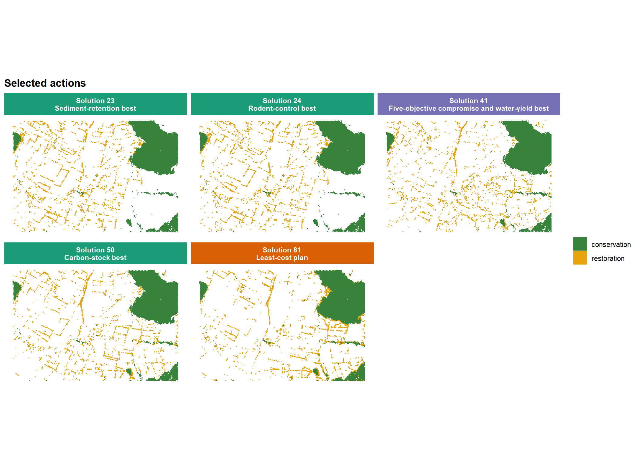
The maps reveal the spatial mechanism behind the objective trade-offs. They show whether improved targeting of a service deficit is achieved through a small number of local substitutions or through a broader relocation of the restoration portfolio across the landscape.
Because the conservation network is fixed, all differences among panels arise from the 2,112 restoration decisions. Comparing the service-specific extremes shows whether different deficits point to common restoration areas or to contrasting parts of the productive matrix. The compromise map identifies the allocation that balances these competing spatial signals rather than optimizing one of them in isolation.
Compare decision-space similarity
Two plans can have similar objective values while selecting different places. Jaccard similarity complements the performance diagnostics by measuring overlap in selected planning-unit–action pairs.
The heatmap follows the same cost ordering used above. Higher similarity means that two plans prescribe more of the same spatial actions. Exact duplicate decision vectors have already been removed, so values close to one indicate very similar but not necessarily identical portfolios.
The fixed conservation network contributes the same assignments to every solution and can therefore raise overall similarity. Differences among plans are generated only by the variable restoration component. Consequently, the heatmap should be interpreted as similarity of the complete intervention system in a setting where one large component is intentionally held constant.

Selection frequency provides a more local view of stability. It reports how often each planning-unit–action assignment appears across the retained non-dominated solutions.
For restoration units, a high frequency indicates that a location is selected under many different combinations of cost and ecosystem-service limits. Such a site is comparatively robust to the trade-off configuration explored here. For conservation units, frequency one is expected because those assignments are locked into every solution.
Frequency is therefore a measure of stability within this generated solution set. It should not be interpreted as ecological irreplaceability, restoration success, or the probability that a site is objectively optimal.
  assignment_frequency <- selection_frequency(efficient_solutions)

  head(
    assignment_frequency[
      order(-assignment_frequency$frequency),
    ],
    15
  )
#>        pu       action n_selected n_solutions frequency
#> 83  10075  restoration         16          16         1
#> 109 10099  restoration         16          16         1
#> 196 10180  restoration         16          16         1
#> 198 10182  restoration         16          16         1
#> 226 10208  restoration         16          16         1
#> 227 10209  restoration         16          16         1
#> 283  1026 conservation         16          16         1
#> 338 10314  restoration         16          16         1
#> 387 10360  restoration         16          16         1
#> 388 10361  restoration         16          16         1
#> 646 10605  restoration         16          16         1
#> 651 10610  restoration         16          16         1
#> 786 10736  restoration         16          16         1
#> 840 10786  restoration         16          16         1
#> 978 10919  restoration         16          16         1
Interpretation and limitations
This vignette demonstrates how multiscape can prioritize
additional forest restoration in a highly productive landscape where
land is scarce, existing uses matter, and ecosystem-service deficits are
spatially heterogeneous. The existing conservation network is treated as
fixed, and every alternative adds the same 2,112 restoration units. The
decision problem is therefore entirely about spatial allocation: which
parts of the productive matrix should be restored?
The formulation gives a specific answer to that question. It favours locations with low implementation cost and low current levels of four ecosystem services. These low-service locations are treated as areas of ecological deficit, making them plausible candidates for restoration while avoiding sites where important functions are already strongly provided. By retaining the services as separate objectives, the model shows that there is no single universal map of ecological need: carbon, water, sediment retention, and biological control can point to different restoration priorities.
This interpretation must remain within the limits of the data and formulation. The deficit effects assume a common service ceiling. Low baseline service provision is not evidence of high realized restoration potential. A degraded site may respond strongly to intervention, weakly, or only after a long time. Conversely, a site with high current service provision could still benefit from restoration. The model identifies where current service deficits and implementation costs favour intervention; it does not predict the ecological response produced by that intervention.
A more complete application could combine the present deficit-based objectives with empirically estimated action outcomes, feasibility, time to recovery, land-use opportunity cost, connectivity, or future climate risk. Those additions would distinguish more explicitly between where services are currently low and where restoration is expected to improve them most.
Finally, the generated alternatives depend on the epsilon design. The 81 requested boundary configurations provide a transparent first exploration of the five-dimensional trade-off space, not an exhaustive approximation of the Pareto frontier. A real decision process should refine the thresholds around policy-relevant regions, test the stability of the spatial recommendations, and use stakeholder input to identify acceptable compromises after the consequences of the alternatives have been made visible.