Plot spatial feature values from a solution set

Plot feature values in space from a solutionset-class object returned by solve.

This function combines baseline feature amounts from the associated Problem object with positive effects induced by the actions selected in each stored run to produce planning-unit-level feature maps. Selected actions are obtained through get_actions.

Usage

plot_spatial_features(
  x,
  runs = NULL,
  features = NULL,
  value = c("final", "baseline", "benefit"),
  layout = NULL,
  max_facets = 4L,
  ...,
  base_alpha = 0.1,
  selected_alpha = 0.9,
  base_fill = "grey92",
  base_color = NA,
  selected_color = NA,
  draw_borders = FALSE,
  show_base = TRUE,
  fill_na = "grey80",
  use_viridis = TRUE
)

Arguments

x

A solutionset-class object returned by solve.

runs

Optional integer vector of run ids. If NULL, the first available run is plotted by default.

features

Optional feature subset to display. Matching is attempted against both feature ids and feature names.

value

Character string indicating which feature quantity to plot. Must be one of "final", "baseline", or "benefit".

layout

Character string controlling the layout. Must be one of "single" or "facet". If NULL, the default is "facet".

max_facets

Maximum number of feature facets shown when features = NULL and faceting would otherwise create many panels.

...

Reserved for future extensions.

base_alpha

Unused in the current feature view, kept for interface consistency.

selected_alpha

Unused in the current feature view, kept for interface consistency.

base_fill

Unused in the current feature view, kept for interface consistency.

base_color

Unused in the current feature view, kept for interface consistency.

selected_color

Border colour for filled feature polygons.

draw_borders

Logical. If FALSE, borders are not drawn.

show_base

Unused in the current feature view, kept for interface consistency.

fill_na

Fill colour for missing values.

use_viridis

Logical. If TRUE and the viridis package is available, use a continuous viridis scale.

Value

Invisibly returns a ggplot object.

Details

For each planning unit \(i\) and feature \(f\), the plotted quantities are: $$ \mathrm{baseline}_{if}, $$ $$ \mathrm{benefit}_{if}, $$ $$ \mathrm{final}_{if} = \mathrm{baseline}_{if} + \mathrm{benefit}_{if}. $$

In the current implementation:

• baseline is the summed baseline amount from dist_features;

• benefit is the summed positive effect from selected actions;

• final is baseline + benefit.

Negative effects are not subtracted in this plotting method. Therefore, value = "final" should be interpreted as baseline plus selected positive effects under the current plotting logic.

If layout = "facet" and only one run is plotted, one panel is drawn per feature.

If multiple runs are plotted, exactly one feature must be requested, and faceting is done by run.

Planning-unit geometry must be available in the associated problem object.

See also

get_features, plot_spatial, plot_spatial_pu, plot_spatial_actions

Examples

if (
  requireNamespace("sf", quietly = TRUE) &&
  requireNamespace("ggplot2", quietly = TRUE) &&
  requireNamespace("rcbc", quietly = TRUE)
) {
  data("sim_pu_sf", package = "multiscape")

  pu <- sim_pu_sf[
    seq_len(min(4L, nrow(sim_pu_sf))),
  ]

  pu$id <- seq_len(nrow(pu))
  pu$cost <- seq_len(nrow(pu))

  features <- data.frame(
    id = 1:2,
    name = c("feature_1", "feature_2")
  )

  dist_features <- data.frame(
    pu = rep(pu$id, each = 2),
    feature = rep(features$id, times = nrow(pu)),
    amount = c(
      4, 1,
      3, 2,
      2, 3,
      1, 4
    )
  )

  actions <- data.frame(
    id = c("conservation", "restoration")
  )

  effects <- data.frame(
    action = rep(actions$id, each = 2),
    feature = rep(features$id, times = 2),
    multiplier = c(
      1.0, 1.0,
      1.5, 1.5
    )
  )

  problem <- create_problem(
    pu = pu,
    features = features,
    dist_features = dist_features,
    cost = "cost"
  ) |>
    add_actions(
      actions = actions,
      cost = c(
        conservation = 1,
        restoration = 2
      )
    ) |>
    add_effects(
      effects = effects,
      effect_type = "after"
    ) |>
    add_constraint_targets_relative(0.25) |>
    add_objective_min_cost(alias = "cost") |>
    set_solver_cbc(verbose = FALSE)

  solutions <- solve(problem)

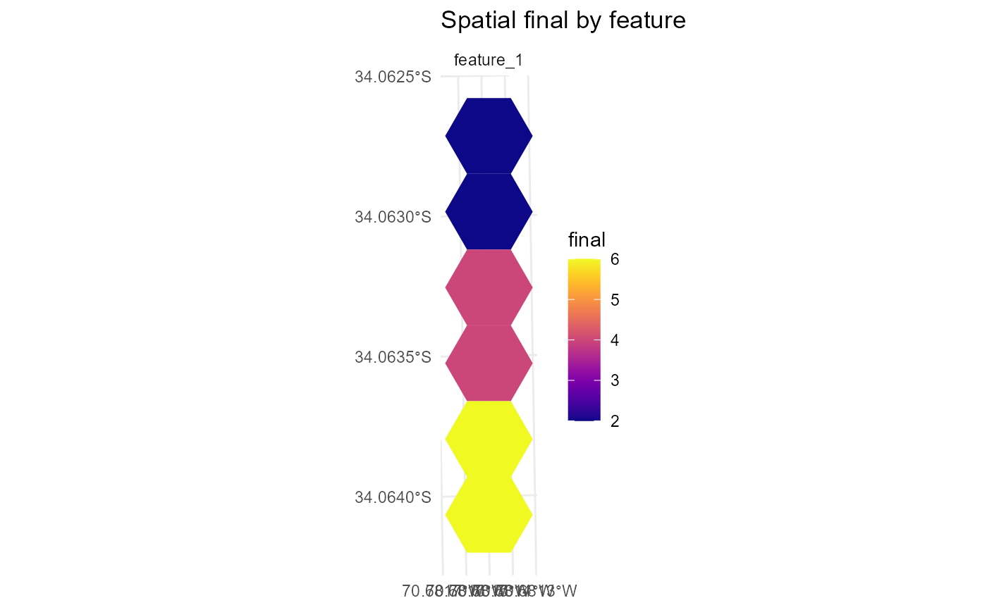
  plot_spatial_features(
    solutions,
    features = "feature_1",
    value = "final"
  )
}