Plot trade-offs from a solution set

Plot pairwise trade-offs among objective values stored in a solutionset-class object.

This function is intended for workflows in which the solution set contains one row per run and two or more objective-value columns of the form value_*.

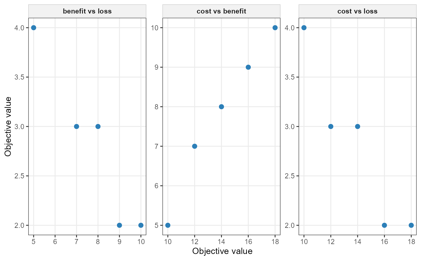
If exactly two objectives are selected, the function returns a single scatterplot. If three or more objectives are selected, all pairwise combinations are plotted using facets.

Usage

plot_tradeoff(
  x,
  objectives = NULL,
  color_by = NULL,
  all_pairs = NULL,
  connect = FALSE,
  label_runs = FALSE,
  point_size = 3,
  line_alpha = 0.5,
  text_size = 3,
  ...
)

Arguments

x: A solutionset-class object.
objectives: Optional character vector of objective aliases to display. These must match the suffixes of the value_* columns in x$solution$runs. If NULL, all available objective columns are used.
color_by: Optional character scalar used to colour points. This may be either one of the selected objective aliases or one of the run-level columns "run_id", "status", "runtime", or "gap".
all_pairs: Logical. If TRUE, allow plotting all pairwise combinations even when more than four objectives are selected. If NULL, it is treated as FALSE.
connect: Logical. If TRUE, connect points by run order within each panel.
label_runs: Logical. If TRUE, add run labels to points.
point_size: Numeric point size.
line_alpha: Numeric alpha value for connecting lines.
text_size: Numeric size for run labels.
...: Reserved for future extensions.

Value

Invisibly returns a ggplot object.

Details

This function reads the run-level table stored in x$solution$runs. It expects objective values to be stored in columns whose names begin with "value_".

If the available objective columns are, for example, value_cost, value_benefit, and value_frag, then the corresponding objective aliases are "cost", "benefit", and "frag".

Let $f_k(r)$ denote the value of objective $k$ in run $r$. This function visualizes pairwise projections of the run table of the form: $$ \left(f_k(r), f_\ell(r)\right) $$ for selected pairs of objectives $k,\ell$.

If exactly two objectives are selected, a single panel is produced.

If three or more objectives are selected, all pairwise combinations are generated: $$ \{(k,\ell): k < \ell,\; k,\ell \in \mathcal{O}\}, $$ where $\mathcal{O}$ is the selected set of objective aliases.

By default, plotting more than four objectives is not allowed unless all_pairs = TRUE, because the number of panels grows quadratically in the number of objectives.

Colouring

If color_by is supplied, points are coloured by either:

one of the selected objective aliases, in which case the corresponding value_* column is used;
or one of the run-level columns run_id, status, runtime, or gap.

Connecting runs

If connect = TRUE, runs are connected in their current table order within each panel. This can be useful when runs correspond to an ordered scan of weights, $\epsilon$-levels, or frontier points, but it should be used with care when run order has no substantive meaning.

Run labels

If label_runs = TRUE, each point is labelled by its run_id. If the ggrepel package is available, repelled labels are used.

Examples

if (
  requireNamespace("ggplot2", quietly = TRUE) &&
  requireNamespace("rcbc", quietly = TRUE)
) {
  pu <- data.frame(
    id = 1:4,
    cost = c(1, 2, 3, 4)
  )

  features <- data.frame(
    id = 1:2,
    name = c("sp1", "sp2")
  )

  dist_features <- data.frame(
    pu = c(1, 1, 2, 3, 4),
    feature = c(1, 2, 2, 1, 2),
    amount = c(5, 2, 3, 4, 1)
  )

  actions <- data.frame(
    id = c("conservation", "restoration")
  )

  effects <- data.frame(
    action = rep(actions$id, each = 2),
    feature = rep(features$id, times = 2),
    multiplier = c(
      1.0, 1.0,
      1.5, 1.5
    )
  )

  problem <- create_problem(
    pu = pu,
    features = features,
    dist_features = dist_features,
    cost = "cost"
  ) |>
    add_actions(
      actions = actions,
      cost = c(
        conservation = 1,
        restoration = 2
      )
    ) |>
    add_effects(
      effects = effects,
      effect_type = "after"
    ) |>
    add_constraint_targets_relative(0.05) |>
    add_objective_min_cost(alias = "cost") |>
    add_objective_max_benefit(alias = "benefit") |>
    set_method_weighted_sum(
      aliases = c("cost", "benefit"),
      runs = run_grid(
        n = 3,
        include_extremes = TRUE
      ),
      normalize_weights = TRUE
    ) |>
    set_solver_cbc(verbose = FALSE)

  solutions <- solve(problem)

  plot_tradeoff(
    solutions,
    objectives = c("cost", "benefit")
  )
}

Usage

Arguments

Value

Details

See also

Examples